📨 ZIP Code 📬

A hands-on R session on Zero-Inflated Poisson and other models for rare primate behaviors

João d’Oliveira Coelho

2025-04-02

Why count data is different

• Count data is discrete, non-negative, often skewed
• Examples in primatology:
  • Vocalization frequencies in vervets (few 0s)
  • Tool use occurrences in chimpanzees (some 0s)
  • Bipedalism bouts in chacma baboons (many 0s)
• Why not use linear regression?
  • Violations of assumptions: non-normality, non-constant variance

• Count data is fundamentally different from continuous data and requires specialized statistical treatment.

1. It’s discrete: We’re dealing with whole numbers (0, 1, 2…), not fractions like height or weight.

2. It’s non-negative: You can’t have negative counts, which breaks the assumptions of normal distributions.

3. It’s often skewed: Most counts are low (or even zero), while high counts are more unlikely.

In primate behavior research, count data shows up everywhere—like tracking how often an animal is aggressive or how often it is grooming another individual. Here are some examples, and obviously if you are observing and recording behaviours like these, you will get some zeros or maybe even a lot of zeros.

So you can’t just grab your dataset with a dependent count variable and run a linear regression on top:

• Why? Well, linear Regression assumes normality, but count data violates that assumption.
• Heteros kedasti city: In count data, variance often increases with the mean.
• A standard linear model can predict impossible values (e.g., negative counts), which doesn’t make sense biologically or in real-world scenarios.

The Poisson distribution

• Poisson models count data where mean = variance
• Probability mass function: \[ P(Y = k) = \frac{\lambda^k e^{-\lambda}}{k!} \]
• Example I wanted: capuchin predation events
• Example you get: Salamanders {glmmTMB} dataset

Price SJ, Muncy BL, Bonner SJ, Drayer AN, Barton CD (2016) Effects of mountaintop removal mining and valley filling on the occupancy and abundance of stream salamanders. Journal of Applied Ecology 53 459–468. doi:10.1111/1365-2664.12585

• Instead of linear regression, we need a model designed for count data. The Poisson distribution is the starting point because it naturally describes count-based outcomes.
  
• However, Poisson has strict assumptions (mean = variance), which can be too limiting.

Suppose we’re studying how often capuchins hunt small vertebrates.

This formula calculates the probability of observing exactly k predation events, given an expected rate𝜆. While λ represents both the mean and the variance in a Poisson process.

If hunting events are randomly distributed over time, we could model the number of monthly predation events using a Poisson distribution. I wanted originally to do a hands-on R session with a capuchin predation dataset that we have, but the paper is not yet published so we need to use a publicly available dataset instead.

Thankfully we have the very clean Salamanders dataset from the glmmTMB package. Which are not primates, but show the same ecological and mathematical proprieties for the purpose of learning how to model count data.

The dataset includes salamander counts in different habitats and you can read more about it in this 2016 paper by Price and colleagues.

The Poisson distribution (simulation)

lambda <- 2  # Mean and variance
pois_sample <- rpois(1000, lambda) # Random generation of Poisson distribution
ggplot(data.frame(pois_sample), aes(x = as.factor(pois_sample))) + 
  geom_histogram(stat = "count") + theme_minimal()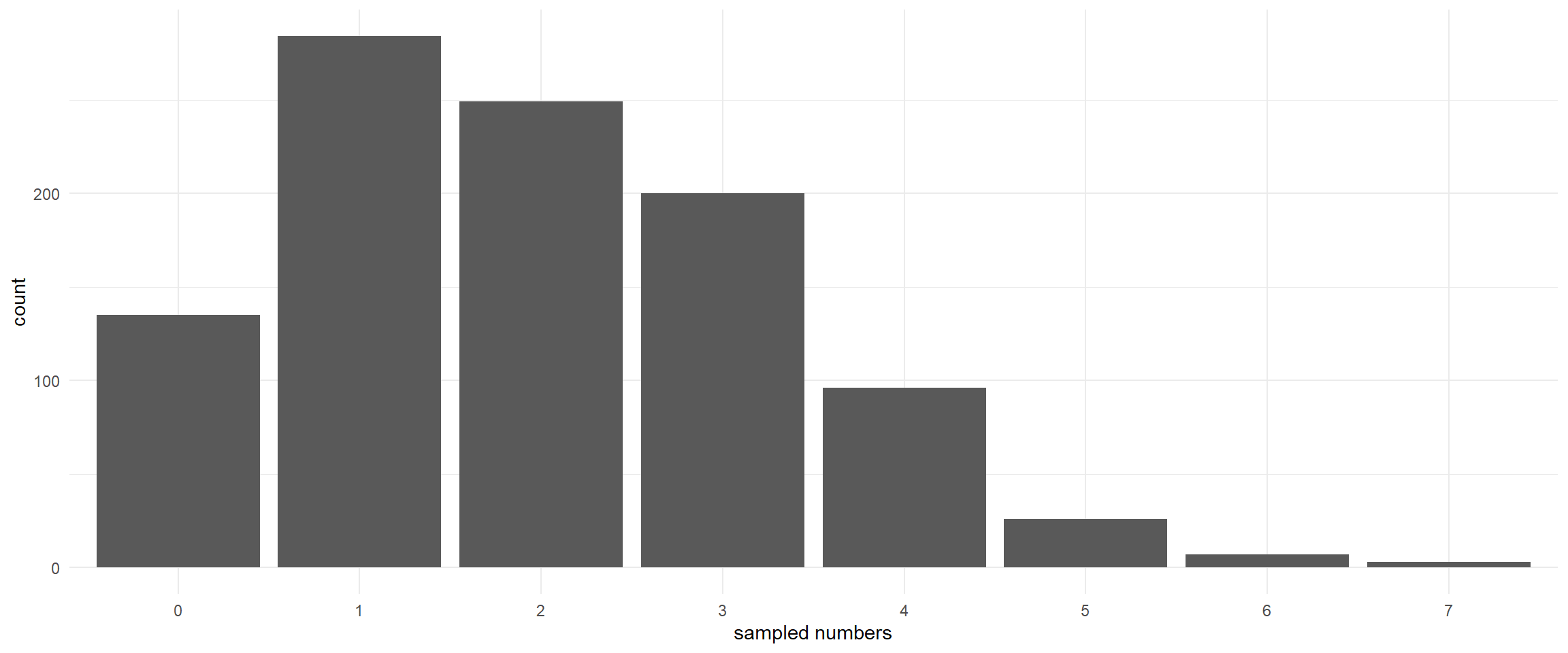

So, if we ask R to generate 1000 random numbers for the Poisson distribution with parameter lambda of 2, we get this histogram. And as you can see, a typical feature of right-skewed distributions is that the mode is to the left of the mean.

Salamander dataset

# Install if necessary
install.packages(c("glmmTMB", "ggplot2", "DHARMa"))

# Load libraries
library(glmmTMB) # For modeling
library(ggplot2) # For visualizations
library(DHARMa)  # For residual diagnostics

data(Salamanders)
str(Salamanders)

'data.frame':   644 obs. of  9 variables:
 $ site  : Ord.factor w/ 23 levels "R-1"<"R-2"<"R-3"<..: 13 14 15 1 2 3 4 5 6 7 ...
 $ mined : Factor w/ 2 levels "yes","no": 1 1 1 2 2 2 2 2 2 2 ...
 $ cover : num  -1.442 0.298 0.398 -0.448 0.597 ...
 $ sample: int  1 1 1 1 1 1 1 1 1 1 ...
 $ DOP   : num  -0.596 -0.596 -1.191 0 0.596 ...
 $ Wtemp : num  -1.2294 0.0848 1.0142 -3.0234 -0.1443 ...
 $ DOY   : num  -1.497 -1.497 -1.294 -2.712 -0.687 ...
 $ spp   : Factor w/ 7 levels "GP","PR","DM",..: 1 1 1 1 1 1 1 1 1 1 ...
 $ count : int  0 0 0 2 2 1 1 2 4 1 ...

Going now to a real dataset, we can use the function structure to quickly have a look at the variables available in the Salamanders dataset.

A data frame with 644 observations on the following 10 variables:

site name of a location where repeated samples were taken

mined factor indicating whether the site was affected by mountain top removal coal mining

cover amount of cover objects in the stream (scaled)

sample repeated sample

DOP Days since precipitation (scaled)

Wtemp water temperature (scaled)

DOY day of year (scaled)

spp abbreviated species name, possibly also life stage

count number of salamanders observed

Salamander dataset (distribution)

sum(Salamanders$count == 0) / nrow(Salamanders)  # Proportion of zeros

[1] 0.6009317

ggplot(Salamanders, aes(x = count)) +
  geom_histogram(binwidth = 1) +
  theme_minimal() + labs(x = "Specimen count", y = "Frequency")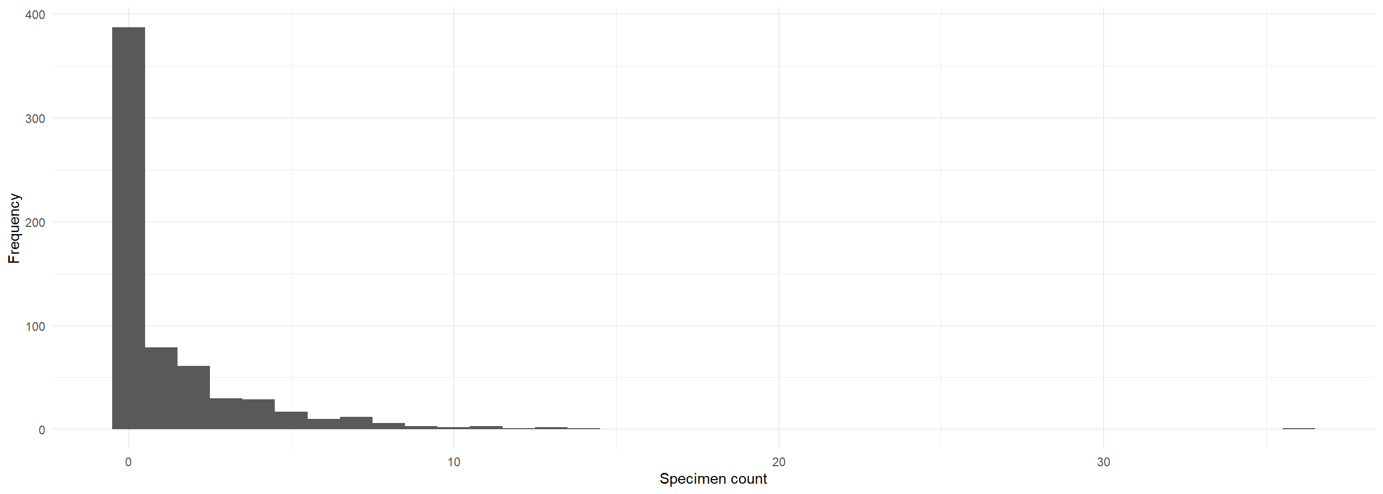

Poisson model

m1_pr <- glmmTMB(count ~ spp + mined + (1|site), data = Salamanders, family = poisson)
summary(m1_pr)

 Family: poisson  ( log )
Formula:          count ~ spp + mined + (1 | site)
Data: Salamanders

     AIC      BIC   logLik deviance df.resid 
  1962.8   2003.0   -972.4   1944.8      635 

Random effects:

Conditional model:
 Groups Name        Variance Std.Dev.
 site   (Intercept) 0.3316   0.5759  
Number of obs: 644, groups:  site, 23

Conditional model:
            Estimate Std. Error z value Pr(>|z|)    
(Intercept) -1.62490    0.24048  -6.757 1.41e-11 ***
sppPR       -1.38626    0.21516  -6.443 1.17e-10 ***
sppDM        0.23054    0.12889   1.789   0.0737 .  
sppEC-A     -0.77010    0.17105  -4.502 6.73e-06 ***
sppEC-L      0.62118    0.11931   5.207 1.92e-07 ***
sppDES-L     0.67918    0.11813   5.750 8.95e-09 ***
sppDF        0.08005    0.13344   0.600   0.5486    
minedno      2.26444    0.28026   8.080 6.48e-16 ***
---
Signif. codes:  0 '***' 0.001 '**' 0.01 '*' 0.05 '.' 0.1 ' ' 1

A random factor (or random effect) accounts for variation that we expect but don’t want to estimate directly. It helps us model data more realistically by acknowledging that some sources of variation are beyond our main variables of interest.

Diagnosis of the Poisson model

simulateResiduals(m1_pr, plot = TRUE)

This function is from the DHARMa package, which provides diagnostic plots for regression models, especially for count data and zero-inflated models.

• What does simulateResiduals() do? Simulates residuals from the fitted model using parametric bootstrapping.

Compares observed residuals to expected ones under the model.

• How to Detect Overdispersion? Overdispersion means the variance is greater than expected under the Poisson model. In DHARMa residual plots, you can spot overdispersion in two main ways:

• Residual Dispersion Plot (2nd Plot)

If residuals fan out (too much spread), it’s a sign of overdispersion.

• QQ Plot (1st Plot)

If points deviate strongly from the 1:1 line, the model is struggling.

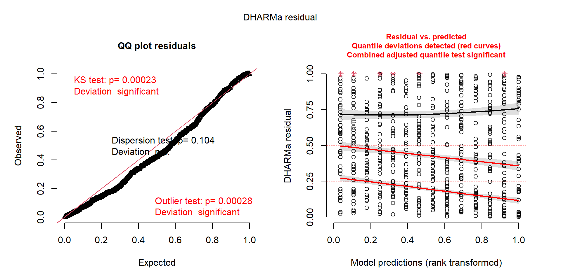
How to handle overdispersion?

• Overdispersion: Variance > Mean
• Poisson assumption often fails → underestimates SE, misleading p-values
• Negative Binomial adds a dispersion parameter to correct for this

• The Poisson distribution assumes that the variance equals the mean, but in real-world ecological data, variance is often greater than the mean.
• When this happens, a Poisson model underestimates standard errors, which in turn leads to misleading confidence intervals and p-values.
• This issue is called overdispersion, and it’s very common in count data, especially in ecological and behavioral datasets.
• Negative Binomial regression is a flexible alternative that includes an extra dispersion parameter, allowing the variance to exceed the mean.
• This dispersion parameter corrects for the overdispersion problem and prevents incorrect statistical inferences.

Negative Binomial model

m2_nb <- glmmTMB(count ~ spp + mined + (1|site), data = Salamanders, family = nbinom2)
summary(m2_nb)

 Family: nbinom2  ( log )
Formula:          count ~ spp + mined + (1 | site)
Data: Salamanders

     AIC      BIC   logLik deviance df.resid 
  1672.4   1717.1   -826.2   1652.4      634 

Random effects:

Conditional model:
 Groups Name        Variance Std.Dev.
 site   (Intercept) 0.2945   0.5426  
Number of obs: 644, groups:  site, 23

Dispersion parameter for nbinom2 family (): 0.942 

Conditional model:
            Estimate Std. Error z value Pr(>|z|)    
(Intercept)  -1.6832     0.2742  -6.140 8.28e-10 ***
sppPR        -1.3197     0.2875  -4.591 4.42e-06 ***
sppDM         0.3686     0.2235   1.649 0.099056 .  
sppEC-A      -0.7098     0.2530  -2.806 0.005017 ** 
sppEC-L       0.5714     0.2191   2.608 0.009105 ** 
sppDES-L      0.7929     0.2166   3.660 0.000252 ***
sppDF         0.3120     0.2329   1.340 0.180337    
minedno       2.2633     0.2838   7.975 1.53e-15 ***
---
Signif. codes:  0 '***' 0.001 '**' 0.01 '*' 0.05 '.' 0.1 ' ' 1

• We will now introduce the Negative Binomial model and compare its fit to our data.

Diagnosis of the Negative Binomial

simulateResiduals(m2_nb, plot = TRUE)

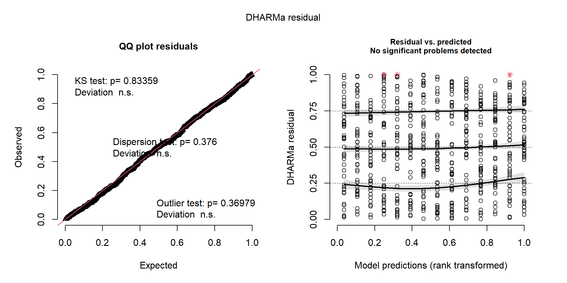
Excess zeros: ZI & hurdle models

• Zero-Inflated models:
  • Some zeros are true, others are structural
  • Zero-Inflated Poisson (ZIP): two processes (occurence)
  • Zero-Inflated Negative Binomial (ZINB): overdispersion
• Hurdle models:
  • Hurdle models are two-part models: 1) classification to detect zeros + 2) regression to model truncated data
  • Here, all zeros are structural

• Many ecological and behavioral datasets contain an excess of zeros—more than would be expected under a standard Poisson or Negative Binomial distribution.
• Some zeros are true: They represent actual absences (e.g., an animal was observed, and the behavior truly did not occur).
• Some zeros are structural: They arise due to underlying processes (e.g., the observer was in the wrong habitat or season where the behavior never occurs).
• Zero-Inflated Poisson (ZIP) models assume that two processes generate the data: one that determines whether a count is zero or not, and another that generates the count itself.
• Zero-Inflated Negative Binomial (ZINB) models extend ZIP by allowing overdispersion in the count-generating process.
• Hurdle models, we do not have time to explore today, but they are really great for rare behaviours and handling excess zeros. They are two-part models → First, a binary model (e.g., logistic regression) predicts whether a zero or non-zero occurs. If non-zero, a truncated count model (e.g., Poisson, Negative Binomial) models the positive counts.
• Key insight: In hurdle models, zeros are always “structural”—they happen because the process doesn’t “cross the hurdle.”

---

Zero-Inflated Poisson model

m3_zip <- glmmTMB(count ~ spp + mined + (1|site), ziformula = ~mined + DOP + Wtemp, 
data = Salamanders, family = poisson)
summary(m3_zip)

 Family: poisson  ( log )
Formula:          count ~ spp + mined + (1 | site)
Zero inflation:         ~mined + DOP + Wtemp
Data: Salamanders

     AIC      BIC   logLik deviance df.resid 
  1798.3   1856.4   -886.2   1772.3      631 

Random effects:

Conditional model:
 Groups Name        Variance Std.Dev.
 site   (Intercept) 0.1281   0.3579  
Number of obs: 644, groups:  site, 23

Conditional model:
            Estimate Std. Error z value Pr(>|z|)    
(Intercept)  -0.4177     0.3009  -1.388  0.16512    
sppPR        -1.2680     0.2408  -5.266 1.39e-07 ***
sppDM         0.2690     0.1377   1.954  0.05074 .  
sppEC-A      -0.5619     0.2050  -2.741  0.00612 ** 
sppEC-L       0.6666     0.1278   5.216 1.83e-07 ***
sppDES-L      0.6229     0.1257   4.955 7.23e-07 ***
sppDF         0.1145     0.1471   0.778  0.43630    
minedno       1.3286     0.2952   4.500 6.79e-06 ***
---
Signif. codes:  0 '***' 0.001 '**' 0.01 '*' 0.05 '.' 0.1 ' ' 1

Zero-inflation model:
            Estimate Std. Error z value Pr(>|z|)    
(Intercept)  0.75729    0.29674   2.552   0.0107 *  
minedno     -1.84122    0.33165  -5.552 2.83e-08 ***
DOP          0.13287    0.12488   1.064   0.2873    
Wtemp       -0.03289    0.12703  -0.259   0.7957    
---
Signif. codes:  0 '***' 0.001 '**' 0.01 '*' 0.05 '.' 0.1 ' ' 1

Zero-Inflated: under the hood

zi_probs <- predict(m3_zip, type = "zprob")  # Probability of excess zeros
ggplot(Salamanders, aes(x = mined, y = zi_probs)) +
  geom_jitter(aes(color = as.factor(count == 0)), width = 0.5, size = 2, alpha = 0.6) +
  stat_summary(fun = mean, geom = "point", color = "black", size = 5) +
  theme_minimal() +
  labs(x = "Mining Presence", y = "Probability of Excess Zeros", color = "Observed Zero?")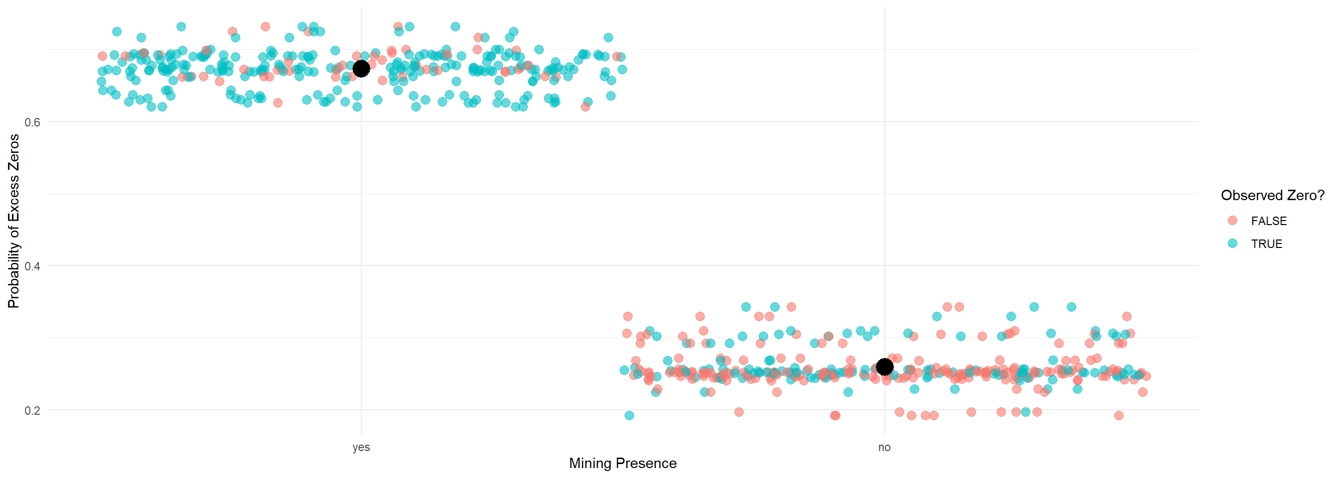

Zero-Inflated Negative Binomial model

m4_zinb <- glmmTMB(count ~ spp + mined + (1|site), ziformula = ~mined + DOP + Wtemp, 
data = Salamanders, family = nbinom2)
summary(m4_zinb)

 Family: nbinom2  ( log )
Formula:          count ~ spp + mined + (1 | site)
Zero inflation:         ~mined + DOP + Wtemp
Data: Salamanders

     AIC      BIC   logLik deviance df.resid 
  1668.0   1730.5   -820.0   1640.0      630 

Random effects:

Conditional model:
 Groups Name        Variance Std.Dev.
 site   (Intercept) 0.1403   0.3745  
Number of obs: 644, groups:  site, 23

Dispersion parameter for nbinom2 family (): 1.05 

Conditional model:
            Estimate Std. Error z value Pr(>|z|)    
(Intercept)  -0.8593     0.3839  -2.238  0.02522 *  
sppPR        -1.3781     0.2860  -4.818 1.45e-06 ***
sppDM         0.3084     0.2261   1.364  0.17260    
sppEC-A      -0.7569     0.2523  -3.000  0.00270 ** 
sppEC-L       0.5388     0.2203   2.445  0.01447 *  
sppDES-L      0.7154     0.2194   3.261  0.00111 ** 
sppDF         0.1720     0.2355   0.730  0.46511    
minedno       1.4999     0.3535   4.242 2.21e-05 ***
---
Signif. codes:  0 '***' 0.001 '**' 0.01 '*' 0.05 '.' 0.1 ' ' 1

Zero-inflation model:
             Estimate Std. Error z value Pr(>|z|)
(Intercept)   -0.3065     0.6593  -0.465    0.642
minedno      -20.5209  3451.8717  -0.006    0.995
DOP           -1.0964     0.7052  -1.555    0.120
Wtemp         -0.2229     0.3414  -0.653    0.514

Model comparison

• Compare models using AIC, residual plots, likelihood ratio tests

anova(m1_pr, m2_nb, m3_zip, m4_zinb, test = "Chisq")

Data: Salamanders
Models:
m1_pr: count ~ spp + mined + (1 | site), zi=~0, disp=~1
m2_nb: count ~ spp + mined + (1 | site), zi=~0, disp=~1
m3_zip: count ~ spp + mined + (1 | site), zi=~mined + DOP + Wtemp, disp=~1
m4_zinb: count ~ spp + mined + (1 | site), zi=~mined + DOP + Wtemp, disp=~1
        Df    AIC    BIC  logLik deviance  Chisq Chi Df Pr(>Chisq)    
m1_pr    9 1962.8 2003.0 -972.40   1944.8                             
m2_nb   10 1672.4 1717.1 -826.20   1652.4 292.40      1     <2e-16 ***
m3_zip  13 1798.3 1856.4 -886.17   1772.3   0.00      3          1    
m4_zinb 14 1668.0 1730.5 -820.00   1640.0 132.35      1     <2e-16 ***
---
Signif. codes:  0 '***' 0.001 '**' 0.01 '*' 0.05 '.' 0.1 ' ' 1

Visualization code

# Generate predictions for all models
Salamanders <- Salamanders %>%
  mutate(
    pred_pr = predict(m1_pr, type = "response"),
    pred_nb = predict(m2_nb, type = "response"),
    pred_zip = predict(m3_zip, type = "response"),
    pred_zinb = predict(m4_zinb, type = "response")
  )

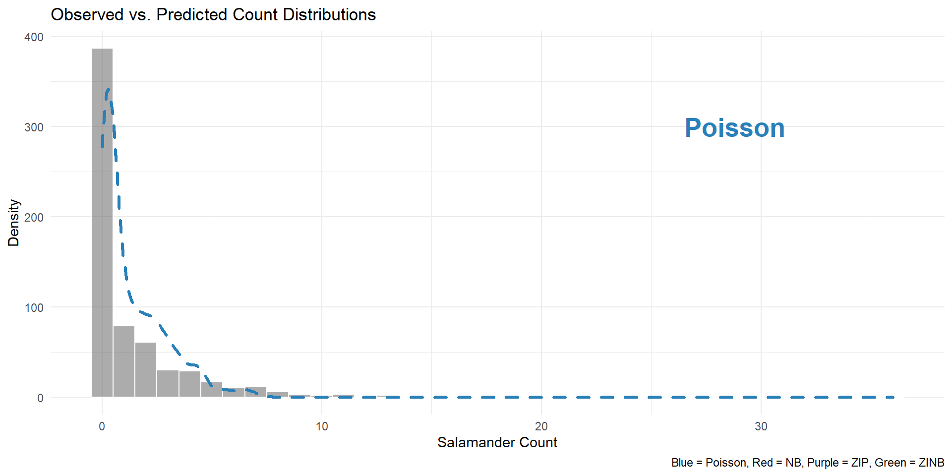
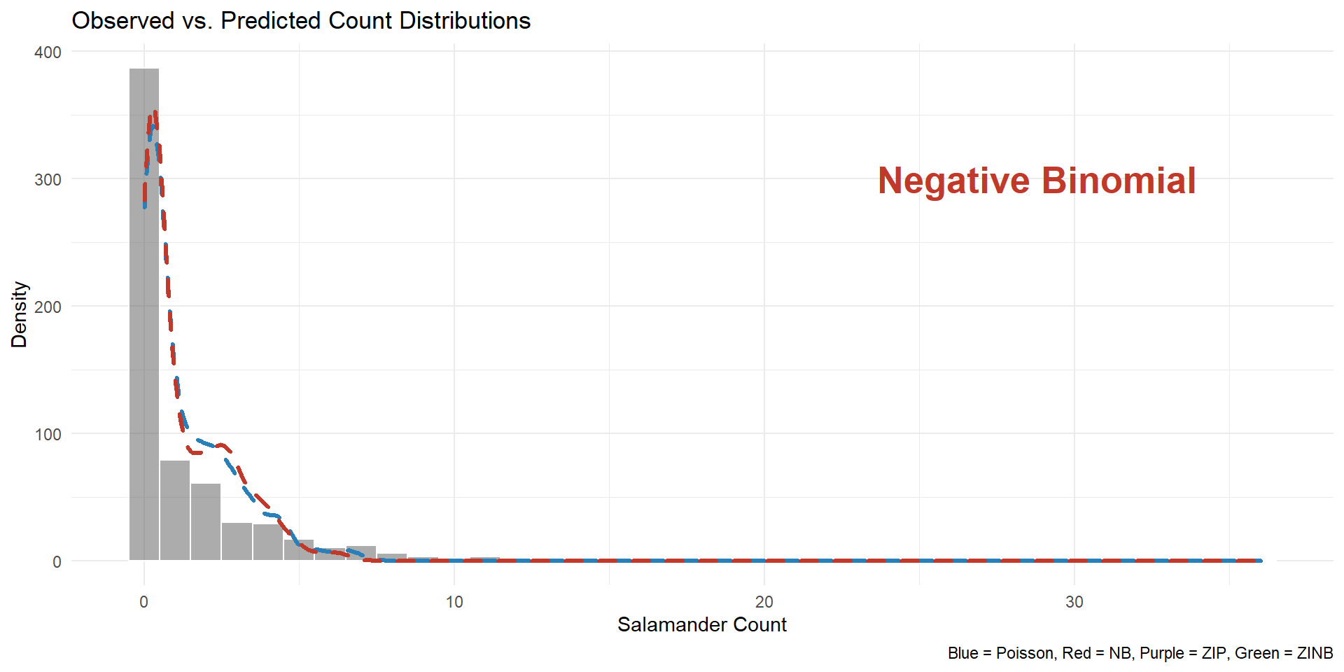
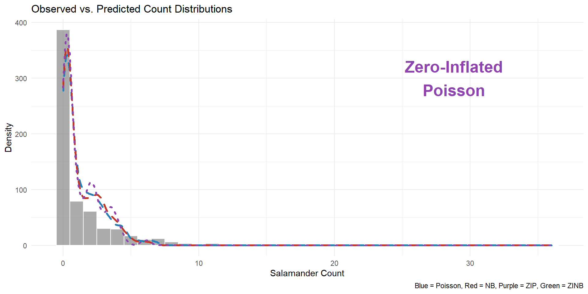
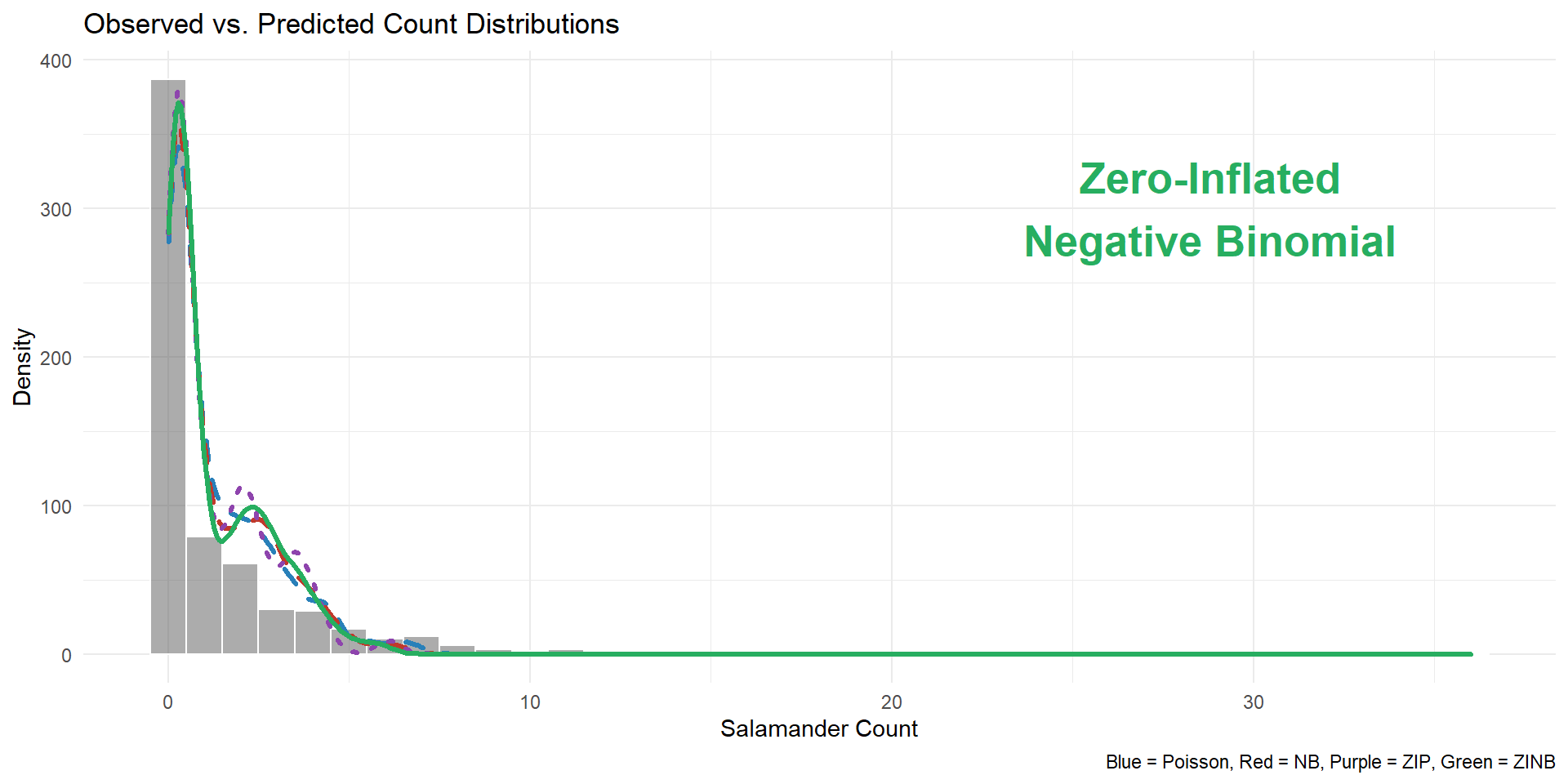
# Plot observed vs. predicted
ggplot(Salamanders, aes(x = count)) +
  geom_histogram(binwidth = 1, alpha = 0.5, color = "white") +
  geom_density(aes(x = pred_pr, y = ..count..), color = "#2980b9", size = 1.2, linetype = "dashed") +
  geom_density(aes(x = pred_nb, y = ..count..), color = "#c0392b", size = 1.2, linetype = "dashed") +
  geom_density(aes(x = pred_zip, y = ..count..), color = "#8e44ad", size = 1.2, linetype = "dotted") +
  geom_density(aes(x = pred_zinb, y = ..count..), color = "#16a085", size = 1.2) +
  theme_minimal() +
  labs(
    title = "Observed vs. Predicted Count Distributions",
    x = "Salamander Count",
    y = "Density",
    caption = "Blue = Poisson, Red = NB, Purple = ZIP, Green = ZINB"
  )

Visualization output

Visualization output

Visualization output

Visualization output

Thank you! Obrigado!

• github.com/Delvis/ZIPcode